MPPI in JAX
From the sampling equations to a controller you can run and change.
Download the uv projectRead the theory notes →
These animations were generated by the JAX implementation with seed 0. Play or scrub through the motion and predicted trajectories. To change parameters and recompute, download the project and run uv run mppi-play.
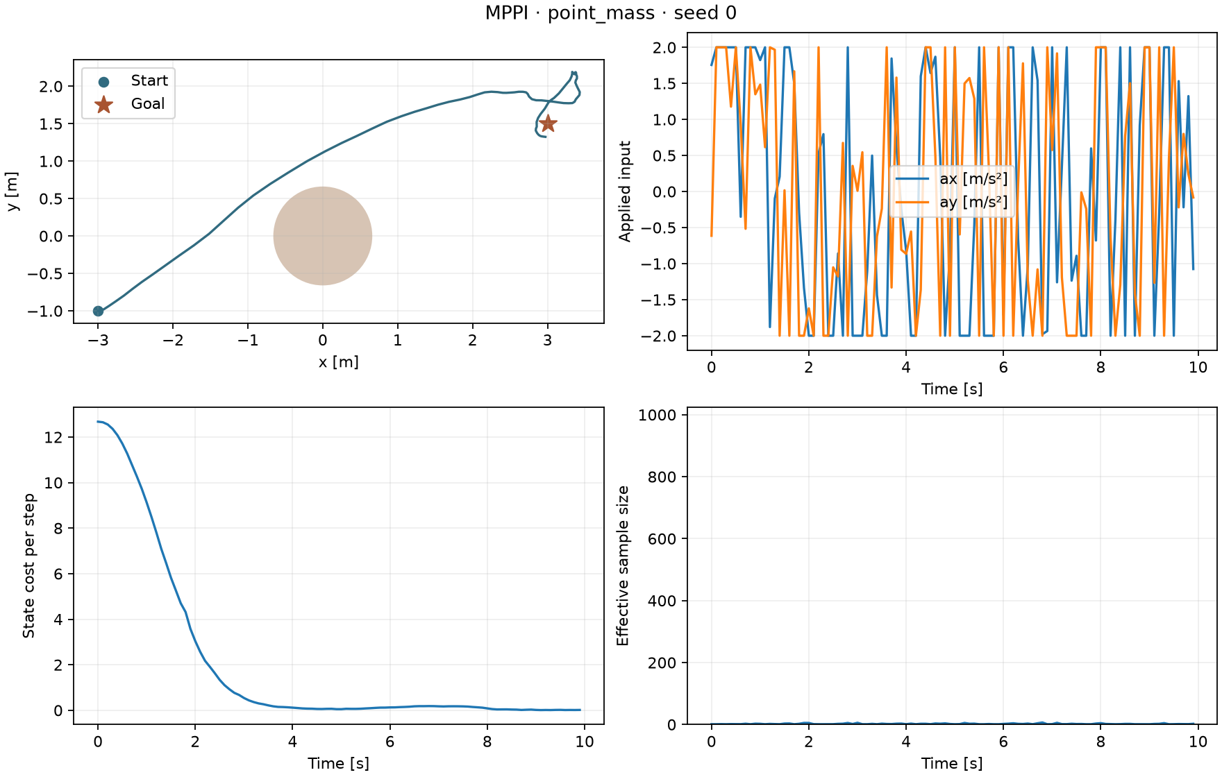 Double integrator →
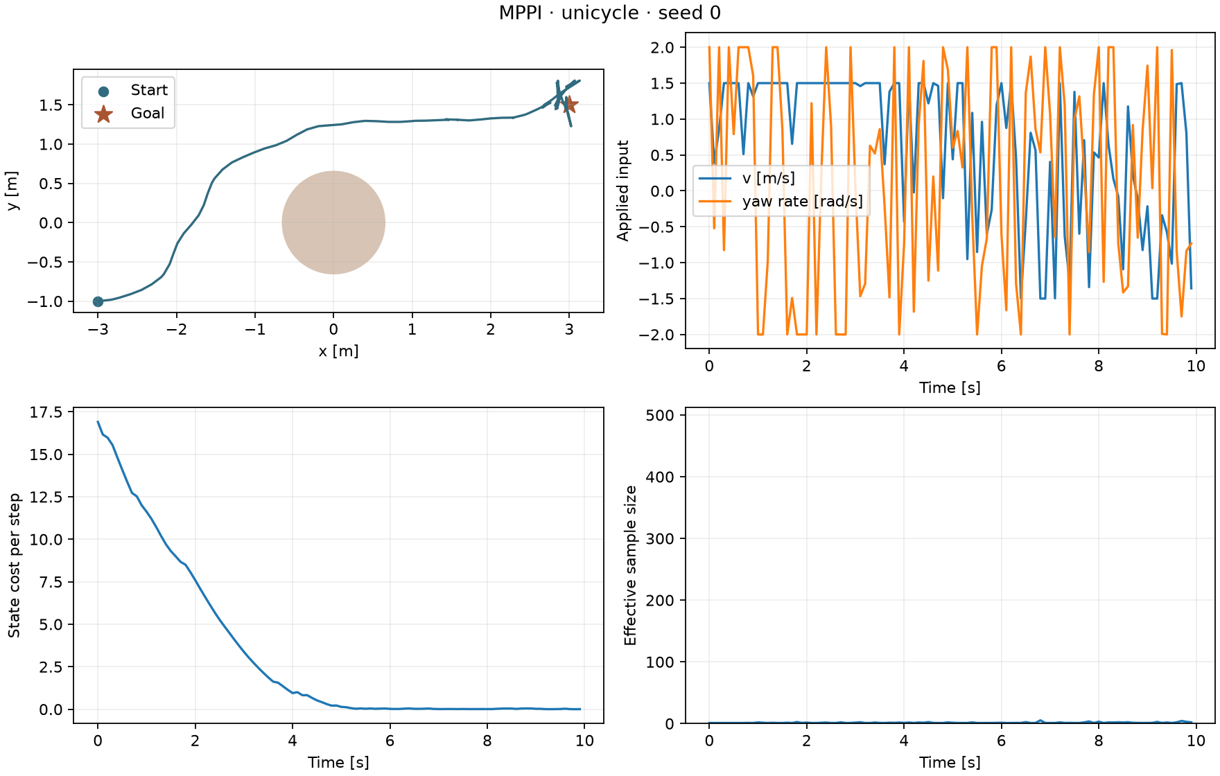 Unicycle →
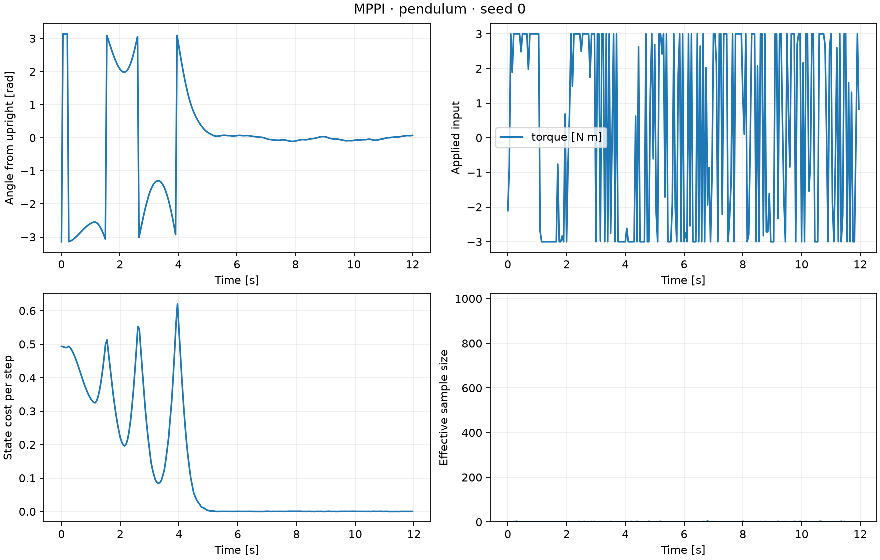 Pendulum swing-up →
This tutorial implements MPPI as a sampling-based method for generating robot trajectories in an MPC loop. The model maps each sampled control sequence to a state trajectory. MPPI evaluates those trajectories and updates the nominal controls using weighted perturbations. The robot executes the first control, and planning repeats from the next measured state.
The MPPI chapter in Kaleb Notes develops the system, the MPC problem, and the method. Its algorithm and block diagram give the full loop before explaining each component. This page maps that loop to a runnable JAX implementation.
The three examples are a double integrator moving around an obstacle, a unicycle moving around an obstacle, and pendulum swing-up. Their models come from the existing notes. The tasks, numerical parameters, and costs are teaching choices. They do not reproduce the papers’ experiments.
1. Install and run with uv
Install uv
using the instructions for your operating system. Download the source
archive, extract it, and open a terminal in its mppi
directory. Then run:
uv sync --locked
uv run mppi-demo --env point_mass --seed 0 --output outputs/point_mass
uv run mppi-demo --env unicycle --seed 0 --output outputs/unicycle
uv run mppi-demo --env pendulum --seed 0 --output outputs/pendulum
If you have access to the source
repository, you can instead clone it and enter
planning-algorithms-library/planning-algorithm-tutorial/mppi
before running the same commands. The public archive does not require
repository access.
Python 3.12 is selected by .python-version. The
committed uv.lock records the dependency versions. The
default JAX installation runs on the CPU; no GPU is required.
Installation needs internet access, but the installed examples and
playback pages do not.
Each run writes four files:
| File | Contents |
|---|---|
playback.html |
Offline animation with play/pause, time slider, predicted paths, inputs, and diagnostics |
summary.png |
Trajectory or angle error, applied inputs, state cost, and effective sample size |
episode.json |
Full settings, seed, software versions, states, actions, predictions, and measured results |
episode.npz |
NumPy arrays for further analysis |
Open playback.html in your browser. For example, on
macOS, run open outputs/point_mass/playback.html. On other
platforms, open the file from your file manager.
For an interactive control panel that runs the actual JAX solver, use:
uv run mppi-playOpen the local playground. It
runs on your machine, bound to the loopback interface. Choose an
environment, change parameters, click Run simulation,
and then play or scrub through the result. Changing the environment
resets its recommended settings. The first run includes compilation.
Press Ctrl+C in the terminal to stop the server. Use
--port 8767 if the default port is occupied.
The published website provides recorded examples; live parameter changes require this local Python process. There is no separate JavaScript approximation of MPPI hidden in the browser.
2. Files and array shapes
| File | Responsibility |
|---|---|
src/jax_mppi/core.py |
Gaussian sampling, rollout, density correction, weights, mean update, and SMPPI |
src/jax_mppi/envs.py |
Models, running state costs, terminal costs, actuator bounds, and default settings |
src/jax_mppi/demo.py |
Receding-horizon loop, experiment records, plots, and command line |
src/jax_mppi/playground.py |
Small local HTTP server calling the same experiment code |
src/jax_mppi/playground.html |
Parameter form and canvas playback |
examples/minimal.py |
A complete controller loop without plotting or the web interface |
examples/compare.py |
Reproducible MPPI/SMPPI comparison across seeds |
tests/ |
Equation-level checks and bounded, reproducible environment runs |
Let \(n\) be the state dimension, \(m\) the input dimension, \(H\) the prediction horizon in steps, and \(K\) the number of sampled sequences. Every state/input vector is represented by a one-dimensional JAX array. The arrays are:
| Python name | Mathematical meaning | Shape |
|---|---|---|
state |
Current measured state \(x_0\) | (n,) |
mean |
Nominal sequence \(\bar U\) before clipping (basic MPPI) | (H, m) |
noise |
Independent perturbations \(E^{(k)}\) | (K, H, m) |
sampled_actions |
Physical control sequences \(U^{(k)}\) | (K, H, m) |
scores,
weights |
Corrected costs \(C_k\) and weights \(w_k\) | (K,) |
predicted |
One rollout, including its initial state | (H + 1, n) |
The prediction index \(t\) runs from
\(0\) to \(H-1\). The sample index \(k\) runs over the batch. We write \(u_t\) for the physical control input and
\(\bar u_t\) for the nominal mean
before clipping. A raw sample is \(\tilde
u_t=\bar u_t+\epsilon_t\). The Python names action
and actions refer to the physical controls \(u_t\) and their sequence \(U\).
3. Define a model and two costs
The controller receives three functions:
step(x, action)       # returns x_next with shape (n,)
state_cost(x)         # returns one scalar c(x_t)
terminal_cost(x)      # returns one scalar phi(x_H)
Use jax.numpy inside these functions. Each function must
return the same array shapes on every call. They should depend only on
their arguments and captured constants. In particular, do not draw NumPy
random numbers or mutate a global object inside a compiled rollout.
The rollout score is
\[S=\sum_{t=0}^{H-1}c(x_t)+\phi(x_H).\]
The code evaluates state_cost before
the state transition, then adds the terminal cost exactly once. If your
cost is a rate per second, multiply it by dt inside
state_cost. The controller does not multiply it a second
time. The terminal cost is not a rate.
Here is the central operation, with output details shortened for explanation:
def advance(x, action):
    cost = state_cost(x)
    x_next = step(x, action)
    return x_next, (x_next, cost)

last, (states, costs) = jax.lax.scan(advance, x0, actions)
total = costs.sum() + terminal_cost(last)
lax.scan carries the current state through the
prediction steps. vmap applies that entire rollout to all
\(K\) action sequences, keeping
x0 shared. jit compiles the calculation for
the selected dimensions. No dynamics or cost derivatives are taken. See
the primary JAX
compilation and vectorization
documentation for those programming operations.
4. Sample input sequences with an explicit random key
The reference covariance is diagonal:
\[\Sigma=\operatorname{diag}(\sigma_1^2,\ldots,\sigma_m^2).\]
config.sigma stores standard
deviations, not variances. covariance_scale stores
\(\nu\), the multiplier in the proposal
covariance \(\nu\Sigma\).
key, draw_key = jax.random.split(key)
noise = jax.random.normal(draw_key, (K, H, m))
noise = noise * sigma * sqrt(nu)
raw = mean[None, :, :] + noise
The controller returns the new key. Reusing the same input key repeats the same draw, so callers must carry the returned key into the next update. Keeping a fixed initial seed makes a complete experiment repeatable on the same software/backend. Bitwise agreement across different accelerators or JAX versions is not assumed. See JAX random keys.
noise_scale on the command line multiplies
sigma, which changes both the reference and proposal.
covariance_scale changes only the proposal and retains the
correction needed for that change.
5. Apply physical input limits without changing the Gaussian algebra
The implementation defines physical actions by
\[u_t=\operatorname{clip}(\tilde u_t,u_{\min},u_{\max}),\qquad \tilde u_t=\bar u_t+\epsilon_t.\]
All rollouts use these bounded controls. The reference and proposal
densities remain densities of the raw Gaussian
variables \(\tilde u_t\). We update
their nominal mean \(\bar u_t\) using
the raw noise, then clip the updated mean to obtain the
physical controls.
This gives a precise interpretation: the task cost is evaluated
through the composite dynamics \(F(x,\operatorname{clip}(\tilde u))\). We do
not pretend that clipped samples still have a Gaussian density. Nor do
we replace noise by clip(mean + noise) - mean
in the density correction.
A consequence is that the mean of clipped samples and the clipped
mean of raw samples need not agree. A bound on physical actions is not a
bound on mean. Inspect both if you change the
controller.
6. Compute the score from the likelihood ratio
Let \(p(\tilde U)=\prod_t\mathcal N(\tilde u_t;0,\Sigma)\) and \(q_{\bar U}(\tilde U)=\prod_t\mathcal N(\tilde u_t;\bar u_t,\nu\Sigma)\). The target is proportional to \(e^{-S(\tilde U)/\lambda}p(\tilde U)\), where \(S\) is evaluated through the clipped controls. Sampling from \(q_{\bar U}\) therefore requires the factor \(p/q_{\bar U}\).
After dropping terms common to every sample, the corrected score is
\[C_k=S_k+\lambda\sum_{t,j}\frac{\bar u_{t,j}\epsilon_{t,j}^{(k)}}{\sigma_j^2} +\frac\lambda2(1-\nu^{-1})\sum_{t,j}\frac{(\epsilon_{t,j}^{(k)})^2}{\sigma_j^2}.\]
Here \(j\) indexes the \(m\) input components. In
corrected_scores:
cross = jnp.sum(mean[None, :, :] * noise / sigma**2, axis=(1, 2))
variance = 0.5 * (1.0 - 1.0 / nu) * jnp.sum(
    (noise / sigma)**2, axis=(1, 2)
)
scores = state_costs + temperature * (cross + variance)
For \(\nu=1\), the last term vanishes. This gives Kim et al., Equation (10). The covariance extension follows the Gaussian likelihood-ratio argument in Williams et al., Section III. The chapter gives the complete expansion, including the terms that cancel.
Do not add an arbitrary quadratic input penalty as a substitute for this correction. An extra cost may be a deliberate new objective, but it does not automatically implement the density ratio.
7. Normalize and update
Compute
\[\beta=\min_k C_k,\qquad w_k=\frac{\exp[-(C_k-\beta)/\lambda]} {\sum_j\exp[-(C_j-\beta)/\lambda]},\qquad \bar u_t^+=\bar u_t+\sum_kw_k\epsilon_t^{(k)}.\]
The minimum subtraction leaves the normalized weights unchanged. It makes the largest exponential equal to one. In code, the sum over samples is
new_mean = mean + jnp.einsum("k,ktm->tm", weights, noise)Every step of one sampled sequence uses that sequence’s weight. The function returns the updated mean, physical actions, scores, weights, and effective sample size \(1/\sum_k w_k^2\).
Nonfinite scores receive zero weight. When every score is nonfinite,
valid is false, the previous plan is preserved, and
run_episode stops before sending a new action. This handles
a numerical failure; it is not a safety controller.
The sample mean is not guaranteed to reduce the deterministic trajectory cost. The reference racing code retains an incumbent or chooses a best sample in some versions; this tutorial deliberately exposes the paper-derived weighted update so the equations and executed algorithm agree.
8. Apply one input, then shift once
result = controller.optimize(key, state, mean, actions)
key = result.key
state = plant_step(state, result.actions[0])
mean = shift_sequence(result.mean)
actions = shift_sequence(result.actions)
Here plant_step = jax.jit(env.step) is created once
before the loop, as in examples/minimal.py.
optimize may perform several updates from the same
state, using fresh samples for each update. It does not shift the
horizon. shift_sequence discards the first entry and
repeats the last entry. In a robot application, replace the simulated
plant step with sending the first action and receiving the next state
estimate.
The demonstration compiles an update separately before timing. It
calls jax.block_until_ready so reported solve times include
completion rather than just dispatch. Reported times include the
requested updates, but exclude plot generation, plant simulation, and
diagnostic prediction. They are measurements on the current machine, not
real-time guarantees.
9. The three environments, fully specified
Double integrator: acceleration-controlled motion
State \(x=(p_x,p_y,v_x,v_y)\);
physical control input \(u=(u_x,u_y)\);
dt = 0.1 s. Each acceleration is bounded to \([-2,2]\) m/s². The exact constant-input
step is
\[p^+=p+\Delta t\,v+\tfrac12\Delta t^2u,\qquad v^+=v+\Delta t\,u.\]
The initial state is \((-3,-1,0,0)\) and the goal is \((3,1.5,0,0)\). Let \(p_g=(3,1.5)\) and let \(B(p)\) be the obstacle cost defined below. The costs are
\[c(x)=\Delta t\,[3\|p-p_g\|^2+0.5\|v\|^2+B(p)], \qquad \phi(x)=25\|p-p_g\|^2+8\|v\|^2.\]
The squared Euclidean norm \(\|z\|^2\) is the sum of the squared components of \(z\). The default uses \(H=25\), \(K=1024\), \(\sigma=(3,3)\), \(\lambda=3\), one update per control step, and 100 executed steps. Goal success means final position error below 0.3 m, speed below 0.5 m/s, and nonnegative measured segment clearance.
Unicycle: velocity and heading-rate commands
State \(x=(p_x,p_y,\theta)\);
physical control input \(u=(v,\omega)\); dt = 0.1 s.
The input bounds are \(v\in[-1.5,1.5]\)
m/s and \(\omega\in[-2,2]\) rad/s.
Reverse motion is allowed. Holding the commands constant, define
\[d=v\Delta t\,\operatorname{sinc}(\omega\Delta t/(2\pi)),\qquad \theta_m=\theta+\omega\Delta t/2,\]
\[p_x^+=p_x+d\cos\theta_m,\quad p_y^+=p_y+d\sin\theta_m, \quad\theta^+=\theta+\omega\Delta t.\]
Here \(\operatorname{sinc}(z)=\sin(\pi
z)/(\pi z)\), with value one at zero, matching
jnp.sinc. This exact step stays well defined at zero
angular rate.
The initial state is \((-3,-1,0)\) and the goal position is \((3,1.5)\). There is no final heading requirement. Costs are \(c(x)=\Delta t[4\|p-p_g\|^2+B(p)]\) and \(\phi(x)=30\|p-p_g\|^2\). Defaults: \(H=40\), \(K=512\), \(\sigma=(1,1.5)\), \(\lambda=0.8\), two updates per step, and 100 steps. Success means final position error below 0.3 m with nonnegative segment clearance.
Both navigation examples have one circular obstacle centered at \((0,0)\), with radius 0.65 m. The radius includes the robot’s size. Define clearance \(d(p)=\|p\|-0.65\). The discrete implementation uses
\[B(p)=1200\max(0,0.35-d(p))^2+2000\,\mathbf 1_{\{d(p)<0\}}.\]
The indicator \(\mathbf 1\) is one inside the obstacle and zero otherwise. The quadratic term starts 0.35 m outside it. These are finite penalties. Collisions remain possible, and averaging obstacle-avoiding input sequences can produce an unsafe mean. The reported minimum clearance checks straight segments between executed positions, not the entire continuous trajectory of the physical system.
Pendulum: swing up with limited torque
State \(x=(\theta,\dot\theta)\), with \(\theta=0\) downward and \(\theta=\pi\) upright. The control input is torque \(u\in[-3,3]\) N m. With mass \(m=1\) kg, length \(l=1\) m, gravity \(g=9.81\) m/s², and damping \(b=0.1\) N m s/rad,
\[\ddot\theta=\frac{u-b\dot\theta-mgl\sin\theta}{ml^2}.\]
The code integrates this equation using classical fourth-order
Runge–Kutta with dt = 0.05 s. For a derivative function
\(f\) and fixed control \(u\), this means \(k_1=f(x,u)\), \(k_2=f(x+\Delta t k_1/2,u)\), \(k_3=f(x+\Delta t k_2/2,u)\), \(k_4=f(x+\Delta t k_3,u)\), and \(x^+=x+\Delta t(k_1+2k_2+2k_3+k_4)/6\).
Define upright angle error \(e=\operatorname{atan2}(\sin(\theta-\pi),\cos(\theta-\pi))\). The costs are
\[c(x)=\Delta t(e^2+0.1\dot\theta^2),\qquad\phi(x)=10e^2+\dot\theta^2.\]
Kim et al., Section IV and Equation (19), use squared angle and angular velocity for swing-up. Here we use the notes’ analytic pendulum model, a downward-zero angle convention, wrapped angle error, and an explicit terminal cost. Their experiment uses learned dynamics; this example does not.
Defaults: \(H=60\), \(K=1024\), \(\sigma=3\), \(\lambda=0.15\), two updates per step, and 240 executed steps from rest downward. Success requires final angle error below 0.2 rad and final angular speed below 0.5 rad/s. The torque is too small for slow direct lifting through every angle, so the controller must build momentum.
10. Compare with smooth MPPI
Run the same environment with a separate physical action sequence:
uv run mppi-demo --env unicycle --mode smppi --seed 0 --output outputs/smppi
uv run python examples/compare.py --seeds 0 1 2 --output outputs/comparison
SMPPI stores a nominal physical control sequence \(\bar U^i\) and a derivative-coordinate mean
\(\bar D^i\). Here \(i\) counts optimization iterations. The
Python array mean stores \(\bar
D^i\) in this mode, while actions stores \(\bar U^i\). Candidate controls are
\[D^{(k)}=\bar D^i+E^{(k)},\qquad U^{(k)}=\operatorname{clip}(\bar U^i+\Delta t\,D^{(k)},u_{\min},u_{\max}).\]
The perturbation covariance is \(\Sigma_d=\operatorname{diag}(\sigma_1^2,\ldots,\sigma_m^2)\) in derivative coordinates, scaled by \(\nu\) for sampling. The score uses the same density-ratio formula with the derivative mean and covariance.
The method adds \(\omega_u\sum_{t=1}^{H-1}\|u_t^{(k)}-u_{t-1}^{(k)}\|^2\)
to the rollout cost, where the scalar smooth_weight is
\(\omega_u\geq0\). This is the
chapter’s matrix weight \(W_u=\omega_u
I_m\), with \(I_m\) the \(m\times m\) identity. The update is
\[\bar D^{i+1}=\bar D^i+\sum_k w_k E^{(k)},\qquad \bar U^{i+1}=\operatorname{clip}(\bar U^i+\Delta t\,\bar D^{i+1},u_{\min},u_{\max}).\]
This is the iteration-indexed update in Kim et al., Equations (15)–(18) and Algorithm 1, with \(u\) reserved for physical controls and \(d\) for derivative coordinates. It is not a cumulative integration along prediction time. The control-difference cost starts at prediction step one and does not include a previously executed control. It provides no hard rate limit. Clipped controls are evaluated in both the rollout and the difference penalty; raw Gaussian derivative perturbations are retained for the density correction.
By default, SMPPI’s derivative standard deviations are the
environment’s action standard deviations divided by dt, so
one candidate perturbation has the same action scale initially. This is
an explicit teaching convention, not a parameter setting copied from the
paper. Tune --noise-scale and --smooth-weight
to explore other choices.
The comparison script reports every requested seed, including failures. It measures final error, task state cost, segment clearance, and the sum of squared changes in executed actions. Smoother actions can come with worse task performance. These toy settings do not establish that one method outperforms another.
11. Experiments to try
Keep the seed fixed while changing one parameter. For example:
uv run mppi-demo --env point_mass --temperature 0.3 --output outputs/cold
uv run mppi-demo --env point_mass --samples 128 --output outputs/fewer
uv run mppi-demo --env point_mass --horizon 10 --output outputs/short
uv run mppi-demo --env point_mass --covariance-scale 1.2 --output outputs/wider
uv run mppi-demo --env pendulum --mode smppi --noise-scale 0.25 --smooth-weight 0.1 --output outputs/smooth_pendulum
Inspect whether the shorter horizon can anticipate the obstacle, whether a smaller batch contains useful motions, and how concentrated weights become. Effective sample size near one means that nearly one trajectory determines the update. Increasing the sample count does not resolve a poorly chosen model or objective. Large covariance changes can also make importance weights concentrate strongly in a long horizon.
The default seed-zero examples reach their stated goal criteria in the recorded CPU run. Other seeds and settings can fail. See validation.json for the complete recorded seed set, configuration, and software/backend information. These are demonstration checks, not a statistical performance study. For seeds 0, 1, and 2, the recorded final-goal results are:
| Environment | MPPI | SMPPI with the shared teaching defaults |
|---|---|---|
| Double integrator | 3 / 3 | 1 / 3 |
| Unicycle | 3 / 3 | 2 / 3 |
| Pendulum | 2 / 3 | 0 / 3 |
All navigation runs in this set had nonnegative measured segment clearance. SMPPI often reduced applied-input variation but did not reliably meet the terminal goal with these settings. The complete records retain both facts. Use the parameter experiments to investigate that tradeoff rather than treating this small table as a ranking of the algorithms.
12. Add your own environment
Begin with examples/minimal.py. Replace the three
model/cost functions, input bounds, and initial state. Keep state
dimension, input dimension, and output shapes fixed during an
experiment. Ensure every evaluation returns finite values for the inputs
you intend to explore.
A new Environment entry also supplies goal metadata,
plotting labels, and recommended settings. For an arbitrary state
representation, adapt the plotting and success checks as well; those
functions currently know the three supplied tasks. No controller code
needs to change if the same model/cost interface is retained.
When changing physical units, change input standard deviations and
cost weights consistently. Rescaling a cost without rescaling
temperature changes the target weights. For stochastic physical
dynamics, specify how disturbance trajectories are sampled and how their
distribution enters the objective before adding random draws to
step.
13. Check the implementation
uv run pytest -q
uv run ruff check src tests examples tools
The tests independently compute Gaussian log density ratios and compare them with the simplified scores for several proposal covariances. They check a hand-computed weighted update, recover the known mean of a one-dimensional Gaussian target, verify running/terminal cost indexing, and distinguish raw Gaussian updates from clipped-action averages. Additional checks cover random key use, horizon shifting, SMPPI’s iteration-axis update, all-invalid batches, and finite bounded runs for every environment and mode.
The code was structured using the supplied
dual_gtk_drs_racing repository’s MPPI as a reference. Its
module points to the earlier JAX car-racing build_mppi
implementation, which uses lax.scan, vmap, and
jit. See SOURCES.md for exact source locations
and revisions, and the differences from those implementations.
The main differences are consequential: this tutorial includes the Gaussian likelihood correction, leaves perturbations unfiltered, retains the raw sampling coordinates, and exposes the weighted update without an incumbent-selection heuristic. Racing-specific dynamics, safety margins, information costs, and gatekeeper acceptance checks are not part of the toy controller.
References
- Grady Williams, Andrew Aldrich, and Evangelos A. Theodorou. Model Predictive Path Integral Control using Covariance Variable Importance Sampling. Supplied arXiv:1509.01149v3, Sections II–IV.
- Grady Williams, Andrew Aldrich, and Evangelos A. Theodorou. Model Predictive Path Integral Control: From Theory to Parallel Computation. 2017. DOI: 10.2514/1.G001921, Sections II, III, and V.
- Taekyung Kim, Gyuhyun Park, Kiho Kwak, Jihwan Bae, and Wonsuk Lee. Smooth Model Predictive Path Integral Control without Smoothing. 2022; supplied arXiv:2112.09988v8. DOI: 10.1109/LRA.2022.3192800, Equations (1)–(19).
The uv project documentation describes the environment and lockfile commands used above. The algorithmic sources are the three supplied papers; the JAX and uv links document software usage.